


What is apparent resistivity?
Whether our focus is on exploring oil and gas reserves, assessing groundwater reservoirs, or identifying geological hazards, electrical surveying stands as an indispensable tool in our toolkit. At the heart of this technique lies apparent resistivity, a pivotal parameter offering essential insights into the makeup and configuration of subsurface layers.
Apparent Resistivity Defining
Apparent resistivity quantifies the resistance of subsurface materials to electrical current flow. During electrical surveys, we introduce current into the ground and measure the resulting voltage. Through analysis of the interplay between injected current and measured voltage, apparent resistivity can be calculated.
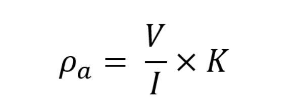
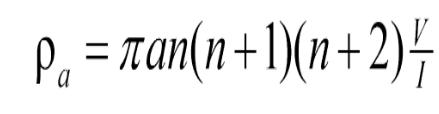
Apparent resistivity (ρa) incorporates the volume of the Earth surrounding the electrodes in resistivity investigations by applying a geometrical factor, Κ, to the determined resistance:
It’s important to note that apparent resistivity is not the same as true resistivity. True resistivity is an inherent property of the formation and remains constant regardless of measurement conditions. In contrast, apparent resistivity is influenced by factors such as the size and shape of the survey area, the spacing between electrodes, and the presence of nearby conductive or resistive features.
Factors affecting apparent resistivity measurements
The key factors affecting apparent resistivity measurements include surface anomalies such as differences in conductivity due to buried utilities, voids, or moisture variation. The nature of the underground materials, including porosity, lithology, and mineral content, also significantly influences these measurements.
Moreover, environmental conditions like temperature, humidity, and soil composition can alter readings and affect the accuracy of apparent resistility data.
Methods for measuring apparent resistivity
There are several methods for measuring apparent resistivity in geophysical surveys.
Some common methods include:
Wenner Array
In this method, four electrodes are placed in a straight line with equal spacing between them. A current is injected through the outer electrodes, and the resulting potential difference is measured between the inner electrodes. Apparent resistivity is calculated based on the geometry of the array and the measured voltage.
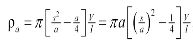
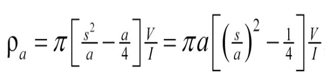
Schlumberger Array
Similar to the Wenner array, the Schlumberger array also uses four electrodes but with varying spacing between them. By adjusting the electrode spacing, this method allows for measurements at different depths, providing a more detailed profile of subsurface resistivity.
Dipole-Dipole Array
This method involves placing two current electrodes and two potential electrodes in a linear array with fixed spacing between them. The distance between the current electrodes is gradually increased, allowing for measurements at different depths. The apparent resistivity is calculated based on the voltage measurements at different electrode spacings.
Self-Potential (SP) Method
While not directly measuring resistivity, the SP method detects natural electrical potentials generated by subsurface electrochemical processes. Changes in SP anomalies can provide indirect information about subsurface resistivity variations.
These methods vary in their sensitivity to different subsurface structures and their suitability for specific survey objectives. The choice of method depends on factors such as the desired depth of investigation, geological conditions, and available equipment.
Additionally, advanced techniques such as tomographic inversion algorithms can be employed to reconstruct 3D resistivity models from multiple apparent resistivity measurements, providing a more comprehensive understanding of subsurface properties.
Related Product:
* ERT Cable: https://www.seis-tech.com/ert-cables-for-abem-instruments/
* Resistivity Cable: https://www.seis-tech.com/resistivity-cable/
* Marine Resistivity Cable: https://www.seis-tech.com/marine-resistivity-cable/
* ABEM LUND Connector: https://www.seis-tech.com/abem-lund-cable-connector/
* Cable Jumper: https://www.seis-tech.com/cable-jumper/
* Non Polarizable Electrode: https://www.seis-tech.com/non-polarizable-electrode-np-60-plus/


